Indexing Techniques

Need for Indexing

Increase performance in terms of a large factor

Goal

Increase efficiency of data access by reducing the number of I/Os required to find desired record(s)​

Catch

It is not always that indexing will save us cost, it might overshoot our cost in scenarios when we have a poor indexing

Cost

• Cost is a combination of finding / accessing the right index and accessing the base table rows lead by those indexes

  $$IndexAccessCost+BaseTableAccessCost$$

  • The Index Access Cost​​ relies on the technique we search the index

    • Binary Search
    • Hashing

  • ​Base Table Access Cost​ is added if access to be table is actually needed

    • A scenario could be when only count is required thus accessing table is not required

• Qualifying rows should be less than the total number of blocks in the table

We can utilise indexing techniques in a number of ways

Criteria for Indexing

• The tables / relations should be large in size

• The table’s update rate should be really low

  • So we can avoid high index updating costs

• The frequency of table access should be high enough

B-Tree Indexing

Type of indexing where we store indexes in a balanced binary sorted tree, in this way we can avoid the cost of of finding the index to just the height of the tree

How Database B-Tree Indexing Works

Cost

$$\log n$$

Where n​ is the number of nodes until the required index value, total height of tree in worst case

Hash Indexing

Index entry in the index table is located by hashing index value

Index entry contains Row ID​ values for each row corresponding to the index value

• Row IDs kept in sorted order to facilitate maximum I/O performance

Build Input

Table that is used in hash table construction

It could be the table that is able to fit into the memory

Probe Input

Table that is used to search into the hash table

We will take the input into our Hash function from this table and reach the corresponding index in the build input

Clustered Indexing

A clustered index is as same as a dictionary where the data is arranged in alphabetical order

There is a consecutive appearance of rows according to the indexed criteria

Clustered Indexes are also called Primary Indexes in some DBMSs however, if the column / file is ordered but that column is not a unique key then that column can be a suitable candidate for forming a clustered index.

• Reduced Cost
• Only one clustered indexing can be performed on one table

The table of contents of books are basically Clustering Indexes

Unique Primary Indexing (UPI)

The column on which indexing is performed is entirely unique

Example

• ​Customer-ID​ in a customer table

Non-Unique Primary Indexing (NUPI)

The column on which indexing is performed might contain duplicates

Example

• ​Account #​ in transaction table

Cost

Clustered Indexes are really fast as compared to non-clustered indexes but we can only create a Clustered Index on a single Column of our table.

The reason they are fast is because consecutive rows are stored according to the indexed column in the base table and thus a Block have more related data to our query.

Single I/O operation for accessing a data row via UPI.

Single I/O operation for accessing a data row via NUPI whenever all rows with the same PI value fit into a single block.

Non-Clustered Indexes

​​

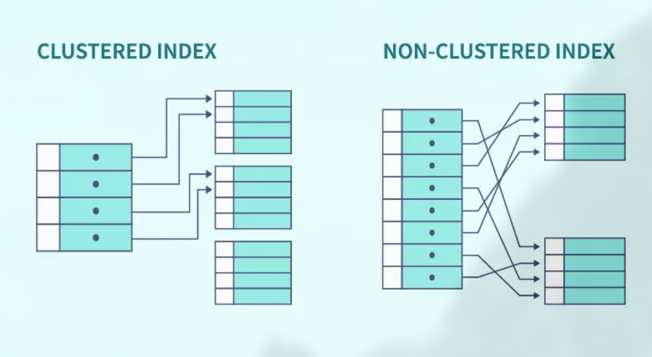
There is no consecutive appearance of rows according to the indexed criteria

Secondary Indexes are also called Non-Clustered Indexes in some DBMSs

• Multiple non-clustered indexing can be performed on one table
• Can only be more than 1 - as in case of Secondary Index

Unique Secondary Indexing (USI)

The column on which indexing is performed is entirely unique

Non-Unique Secondary Indexing (NUSI)

The column on which indexing is performed might contain duplicates

Cost

• Unlike a primary index, secondary indexes are not “free” in terms of storage

Static Bitmap Indexes

Indexes are stored as a Bitmap

• Each bit in a bitmap represents the rows in the table

• For each unique value a bitmap is stored representing the existence of that value in corresponding rows

• For Example, Consider Static Bitmap Indexing on Department Column of a table with 6​ rows and 3​ unique departments
  The indexing will be represented as:

  • HR: 100001
  • IT: 010110
  • Finance: 001000

Therefore, the more the distinct values the more the cost of static bitmap indexes

Best for Low Selectivity Queries

Combining Multiple Indexes

• Indexes Transferred to Memory
• Sorting Operation
• Combining the Index / Intersection

Base Table Cost

Static Bitmap Indexes do not require Base Table Access Cost if only count of rows is required

Dynamic Bitmap Indexes

Index Bitmaps are created at runtime, hence stored in memory

• Same Bitmaps as in the case of Static Bitmap Indexes

Drawback

Bitmaps might have false positives same as in the case of Hash collisions in Hashing

Reasons for False Positives:

• Updates and Deletions: When rows are updated or deleted in the underlying table, the corresponding bitmap indexes must be updated. During this update process, false positives may occur if the bitmap is not perfectly synchronised with the actual data.
• Concurrency Issues: In multi-user environments with concurrent transactions, there can be scenarios where multiple transactions are updating the same bitmap simultaneously, leading to temporary inconsistencies.

Solution: Verify False Positives by accessing the Base Table

Combining Multiple Indexes

• No Copying to memory is Required
• Bitmaps are created at runtime in the memory from the indexed tables and those bitmaps are brought it into the memory and thus avoiding the I/O Cost
• Sorting Cost is avoided, bitmaps comparison are really fast as compared to row comparison

CPU utilisation is less but I/O Cost is the same as in the case of Standard Combining Multiple Indexes

Base Table Cost

Dynamic Bitmap Indexes do require Base Table Access Cost if only count of rows is required, as the bitmaps are created at runtime and thus table need to be browsed

Due to false indexing of Dynamic Bitmap Indexing, we need to scan base table to confirm if the conditions are satisfied on the indexed bitmaps

Dynamic Bitmap Indexes will always access Base table access while Combining Multiple Indexes does not need to visit the Base Table. Therefore Dynamic Bitmap indexes will only be best if we really need to access the Base Table

It is best to apply Dynamic Bitmap Indexes first on low selectivity columns, thus n-1 columns, while one will be the high selectivity column.

Composite Indexing

We will perform combined indexing on more than one columns

This will definitely increase our record size of the indexed table

Efficiency

We need to decide the order of the columns in this type of indexing

Schema should be left to right from Higher Order​ to Lower Order​

The most efficient order will be according to the frequency of access, thus in this way we will avoid reading the unnecessary columns before reading the actual column

Composite Indexing can be extremely efficient if it is designed efficiently

Properties of Indexes

Covered Indexes

Not really a type of indexing but basically a technique through which only entertain those queries that do not need to access the whole base table

i.e. Count of Rows etc.

Dense Indexes

The number of rows are equal to the records in the column

Sparse Indexes

The number of rows will be less than the count of records in the column

Partial Indexes

We will only apply indexing on a special segment of the records in the table

The criteria for this special segment could be the according to the frequency of access etc.

Also known as the 80/20 Rule — Pareto Principle