Join Operations

High Selectivity

Columns or Queries that give us a relatively small result set

• Extremely high selectivity columns are the columns which have the highest discreetness rate

  Example

  IDs, Sr# etc.

• A “highly selective” column leads to a low selectivity value (i.e. low probability of a given row to match the column value)

• A highly selective predicate (one with a selectivity of 0.10 or less) is desirable.

• If Queries they they are more specific
  Example
  A query filtering a row based on some ID

  SELECT *
  FROM CUSTOMER
  WHERE CUSTOMER.ID = 706;

Traditional OLTP Queries

• High Selectivity

Traditional DSS Queries

• Low Selectivity

Techniques

Nested Loop Joins

For every row of an Outer Table, an inner table is searched and joined

Join table T1 to table T2 by taking each (qualifying) row of T1 and searching table T2 for matches

• T1 is referred to as the Outer table

• T2 is referred to as the Inner table

• Simplest form of join algorithm

• No sorting required

Nested loop joins may be fastest join technique when outer table has a small number of qualifying rows and the inner table is very large

Cost

$$O(R\ast S)$$

Where R is the Size of Table 1 and S is the Size of Table 2

This can prove to be quite Costly in terms of huge outer or inner tables

How to avoid Huge Costs

• We can utilise Indexing Techniques to mitigate the cost of finding or browsing though every row

  • Index Nested Loop Joins
  • Clustered Indexed Nested Loop Joins

• Alternatively, the RDBMS can use block nested loop joins to reduce the number of scans against the inner table

  • Block Nested Loop Joins

Break Even Analysis

If we perform indexing to reduce our costs, then the cost can be calculated as:

Outer Table Qualified Rows * (Indexing Retrieval Cost + Avg. Rows in Inner Table for Outer Table Row)

Break even point will be even more optimistic if we assume that substantial portions of the index on the inner table can be cached in memory (first term in round brackets goes to zero) or if a large sort can be avoided.

Usage

• OLTP queries will almost always perform best with a nested loop join

  • This is because OLTP Queries deal with less data and thus less computations

• For traditional DSS queries, high performance with nested loop joins is often dependent on the ability to access through a clustering index

  • This is because the size of data is very huge and clustering index offers physical storage on index value

Sort Merge Join

​​

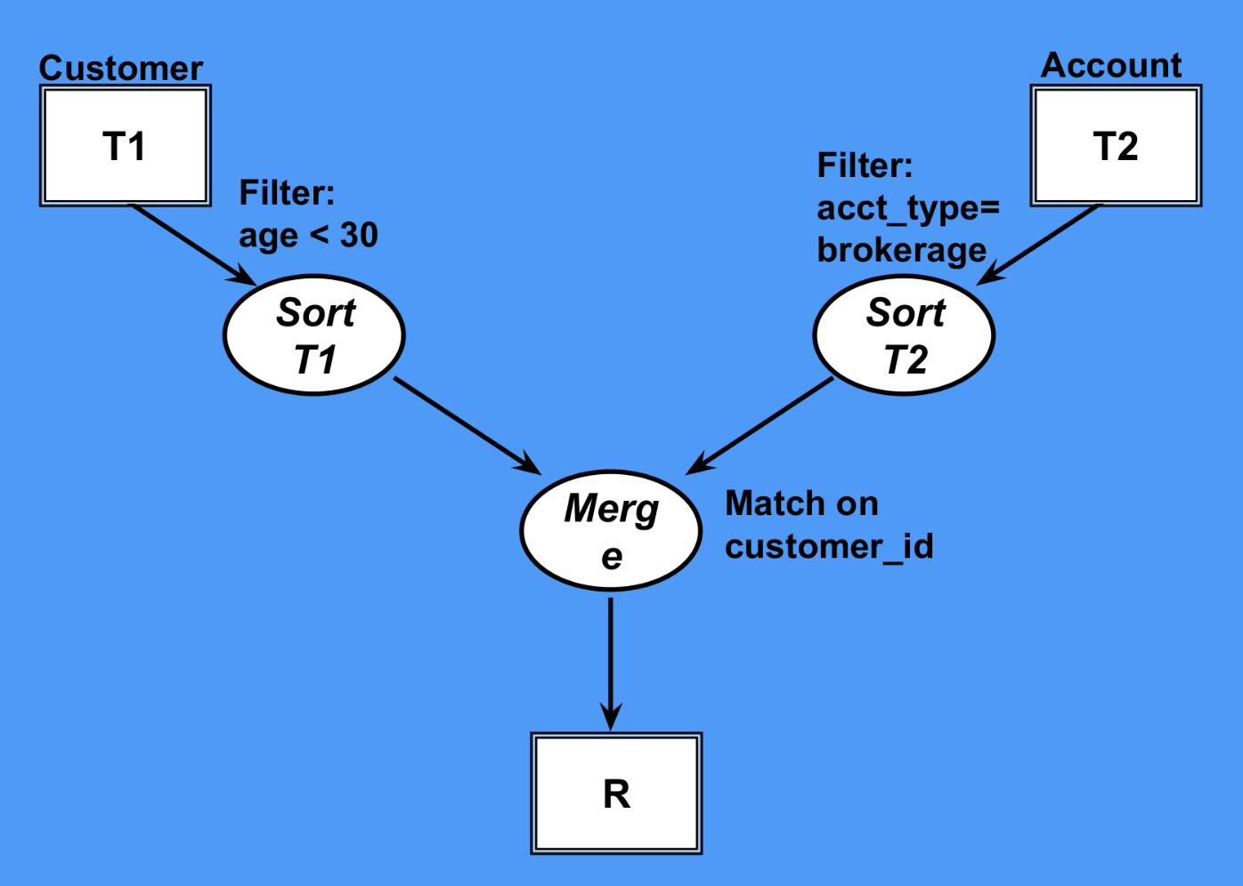
We can sort two tables independently and join them together just as in the case of Merge Sort

External Sorting

Sorting on Disk needs to be performed if memory size is less than the amount of data to sort

Memory Passes

The number of times the table data needs to be brought to memory from the disk

If we have K as our memory and N as our input size and K $\le$ N then we need to bring the data $\frac{N}{K}$ times into the memory. Hence in this case, $\frac{N}{K}$ will be our number of passes.

Cost

$$O(R\ast log\frac{R}{K})+O(S\ast log\frac{S}{K})+O(R+S)$$

Where R is the size of Table 1, S the size of Table 2 and K the memory Size

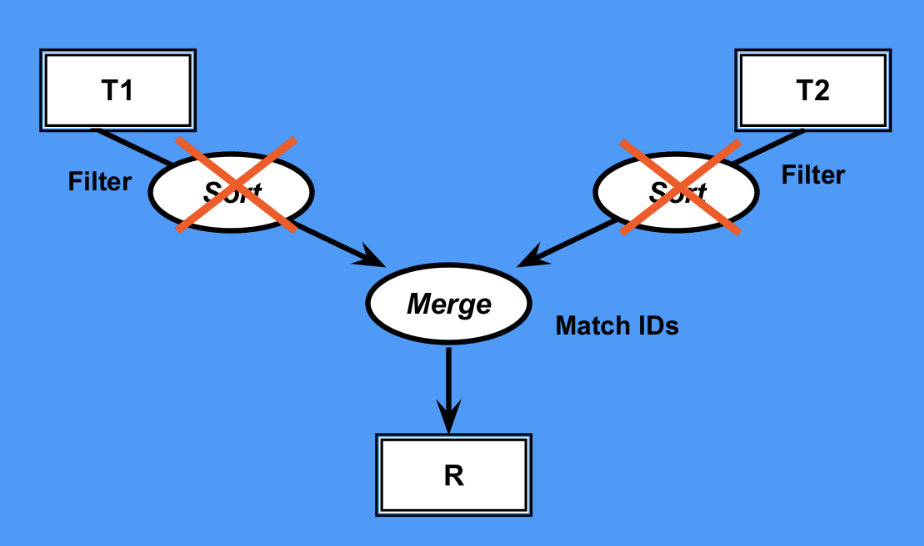
Merge Join

If both table are already sorted then this could be special case of Sort Merge Join in which sorting is already done and thus the only cost is to merge the two sorted tables together

​​

Hash Joins

Join tables by building an in-memory hash table from the smaller of the tables (after considering qualifying rows) and then probing the hash table for matches from the other table

Best Case

If at least one of the table entirely fits into the memory then it’s the best case of Hash Join

• No sorting required
• No need to build any temporary files even when using very large probe input

Cost

$$O(R+S)$$

Where R is the Size of Table 1 and S is the size of Table 2

Worst Case

If both of our tables are not able to fit into the memory. This will be a worst case of Hash join.

We will need to partition both tables into the same size with same joining column data

Cost

$$O(R\ast \log (\frac{R}{K}))+O(S\ast \log (\frac{R}{K}))$$

Where R is the Size of Table 1, S is the size of Table 2 and K is the available memory

The log(R/K) factor arises from the average number of comparisons required to find the hash bucket

Build Input

Table that is used in hash table construction

It could be the table that is able to fit into the memory

Probe Input

Table that is used to search into the hash table

We will take the input into our Hash function from this table and reach the corresponding index in the build input