Storage Structures
Types
- Normalised
- Denormalised
| Normalised Data Structure | Denormalised Data Structure |
|---|---|
| Flexibility | Less Flexibility |
| Low Maintenance Cost | High Maintenance Cost |
| Less Storage Cost | More Storage Cost |
| Low Performance | High Performance |
Criteria to Choose
-
Frequency of Data Access
- If the frequency of access is higher then avoiding the join operator as in going from normalised structure to denormalised structure can be the viable option
Ideal Goal
Provide maximum performance with minimum cost without sacrificing flexibility or usability
Normalisation
1NF
- Atomic Values
- No Repeating Groups
Repeating groups can save space as in the case of denormalised design, however updating existing records is always slower than inserting new records, hence the tradeoff.
2NF
- 1NF and Non Prime Attributes should be fully functionally dependent on the primary key therefore no partial dependencies
Splitting tables as in 2NF can cost us additional joins hence performance bounds but storage will be reduced by getting rid of redundant data, hence the tradeoff
3NF
- 2NF and every Non Prime Attribute should be non-transitively dependent on the primary key therefore no transitive dependencies on the primary key
Performance costs can be our concerns because of additional joins to link entities together but storage costs will be reduced to minimum along with the unified view of the data within the warehouse
Denormalisation
When to implement
- The size of the data is exceptionally large
- The frequency of data access is exceptionally high
Following are the techniques to implement denormalisation:
Pre-Join
Take tables which are frequently joined and “glue” them together into a single table
AKA Join Indexing
- Avoids performance impact of the frequent joins.
- Typically increases storage requirements.
Storage Implications
Assume 1:3 record count ratio between sales header and detail
Assume 1 billion sales (3 billion sales detail)
Assume 8 byte sales_id
Assume 30 byte sales header and 40 byte detail header
Without Denormalisation / Normalisation
- We have two tables one for sales data and other for it’s detail
-
1 Billion Sales x 30 bytes Header = 30 GB -
3 Billion Sales Detail x 40 bytes detail record = 120 GB - ==Total = 150 GB==
With Denormalisation / Without Normalisation
- We will store a total of 3 Billion records in only one table
- However one attribute that is the
sales_id will be redundant so we will deduct it’s size -
3 Billions Sales Data x 30+40-8 Bytes - ==Total = 186 GB==
We have a storage increase of 24% by denormalising. i.e. (186 / 150) -1
Column Replication / Movement
Limited form of Pre-Join
Take columns that are frequently accessed via large scale joins and replicate (or move) them into detail table(s) to avoid join operation
-
Avoids performance impact of the frequent joins
-
Increases storage requirements for database
- However, possible to “move” frequently accessed column to detail instead of replicating it
-
Can achieve table co-location
- Say we want to join three tables we can accomplish that with a single column that is replicated to others
-
Storing a new column every time for a record can increase storage overheads
Pre-Aggregation
Pre Aggregate columns which are accessed on a frequent basis
AKA Aggregate Join Indexing
- Avoids performance impact of the frequent joins
- Increases storage requirements for database
- Aggregates should not replace detailed data
An aggregate table must be used many, many times per day to justify its existence in terms of maintenance overhead in most environments
Dimensional Data Modelling
Dimensional modelling gets its name from the business dimensions we need to incorporate into the logical data model. It is a logical design technique to structure the business dimensions and the metrics that are analysed along these dimensions. This modelling technique is intuitive for that purpose. The model has also proved to provide high performance for queries and analysis
-
Capture Facts / Measures / Metrics
- Such as: Sales, Qty, Sale Amount, Cost etc.
-
View Measures along Dimensions
-
Such as: Time, Store, Product
-
Levels define the scope of the dimensions
- The lowest level is called the grain level
-
Dimensions Levels Time Day, Week, Month, Year Store Store, City, District, Country, Region Product Product, Sub-Category, Category, Department
-
Fact Table
A fact table is a central table in a dimensional data model that captures the quantitative or measurable data about a particular event or business process. It is a key component of a data warehouse or a data mart.
Count of fact tables depend on the business requirements
Cardinality Level
The total number of records in accordance with the dimensional levels in a Fact Table
Types
Fact-less Fact Table
Fact table that contains only the ids of the dimensions instead of facts. It saves us storage overheads on the cost of analysis restrictions, hence the tradeoff.
Base Fact Table
Contains the detailed, transactional-level data. It captures the grain level information related to specific business process or event
| Day | Store | Product | Amount | Qty | Cost | IOH |
|---|
Aggregate Fact Table
An aggregate fact table, on the other hand, contains aggregated or summarised data derived from one or more base fact tables. Aggregations involve combining and summarising the data at a higher level of granularity based on specific dimensions and measures. The purpose of an aggregate fact table is to improve query performance by pre-calculating and storing aggregated values
Aggregate Fact Table can be simple, one-way, two-way, three-way etc based on the aggregation on the number of dimensions
Consider we have three dimensions: Day, Store and Product:
| Day | Store | Product | Amount | Qty | Cost | IOH |
|---|
Simple Aggregate Table
| Month | Country | Amount | Qty | Cost | IOH |
|---|
Simple Aggregate Fact Table - Monthly Sales Country Wise
Not all dimensions are used hence it’s a simple aggregate analysis
Also a 2D Fact Table, since two dimensions are being analysed against all instances of other
One-Way Aggregate Table
| Month | Store | Product | Amount | Qty | Cost | IOH |
|---|
One-Way Aggregate Fact Table - Monthly Sales Product and Store Wise
the day dimension is aggregated into month
| Day | Country | Product | Amount | Qty | Cost | IOH |
|---|
One-Way Aggregate Fact Table - Daily Sales Product and Country Wise
the store dimension is aggregated into country
Two-Way Aggregate Table
| Month | Country | Product | Amount | Qty | Cost | IOH |
|---|
Two-Way Aggregate Fact Table - Monthly Sales Country and Product Wise
the day dimension is aggregated into month
the store dimension is aggregated into country
Three-Way Aggregate Table
| Month | Country | Category | Amount | Qty | Cost | IOH |
|---|
Three-Way Aggregate Fact Table - Monthly Sales Country and Category Wise
the day dimension is aggregated into month
the store dimension is aggregated into country
the product dimension is aggregated into category
Schema Model
A Schema model is used to establish the type of connection between dimensions, fact tables and different levels of dimensions
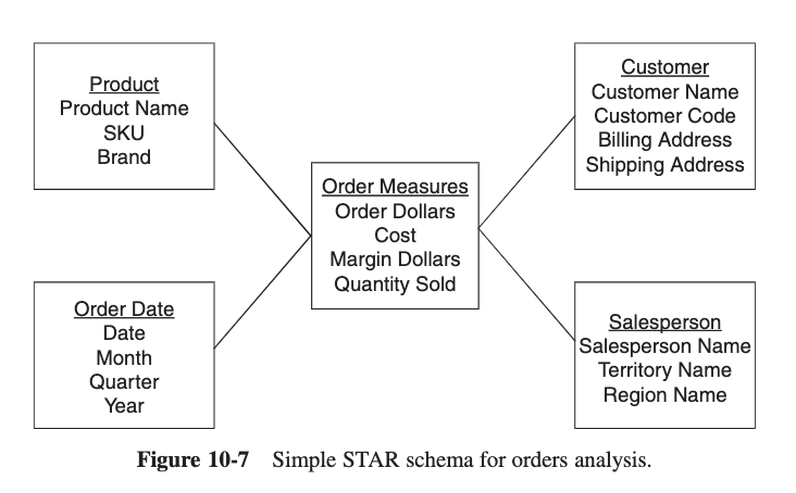
Star Schema
A Star Schema consists of fact tables, dimension tables and establish relationship between each dimension table and the fact table.
Denormalised Structure, therefore huge data redundancies
Fact table resides in the centre while the dimensions connected to it forming a shape of a star
Also See: Drill Down Steps
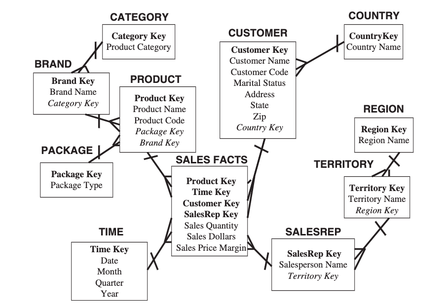
SnowFlake Schema
A Snowflake Schema
Further normalisation of dimensions can lead us to a Snowflake Schema
StarFlake Schema
A starflake schema is a combination of a star schema and a snowflake schema. Starflake schemas are snowflake schemas where only some of the dimension tables have been normalised.
Starflake schemas aim to leverage the benefits of both star schemas and snowflake schemas.