Genomaly

“Genomaly: AI-Powered Image Generation & Anomaly Detection”
An AI-powered system designed to implement and compare different generative AI techniques for anomaly detection in both image and real-world datasets. The project extensively utilizes GANs and VAEs to generate, reconstruct, and identify anomalies across structured and unstructured data. The workflow comprises multiple stages, from exploratory data analysis (EDA) to model training, comparison, and real-world application.

Important

Checkout the section: Save the World with VAE for an industrial anomaly detection implementation in pharmaceutical production within this project.

Part 1: Exploratory Data Analysis

• The training and testing slices for both MNIST Digit and MNIST Fashion datasets were downloaded and analyzed
• A transformation was applied on the images to:
  • Convert them from PIL objects into torch Tensors
  • Normalized them into a range of [-1, 1] (for efficient training later on)
• Both datasets have about 60,000 training and 10,000 testing samples
• Both datasets have 10 class labels:
  • MNIST Digit have class labels: [0, 1, 2, 3, 4, 5, 6, 7, 8, 9]
  • MNIST Fashion also have 10 integral class labels which corresponds to the following classes: [‘T-shirt/top’, ‘Trouser’, ‘Pullover’, ‘Dress’, ‘Coat’, ‘Sandal’, ‘Shirt’, ‘Sneaker’, ‘Bag’, ‘Ankle boot’]

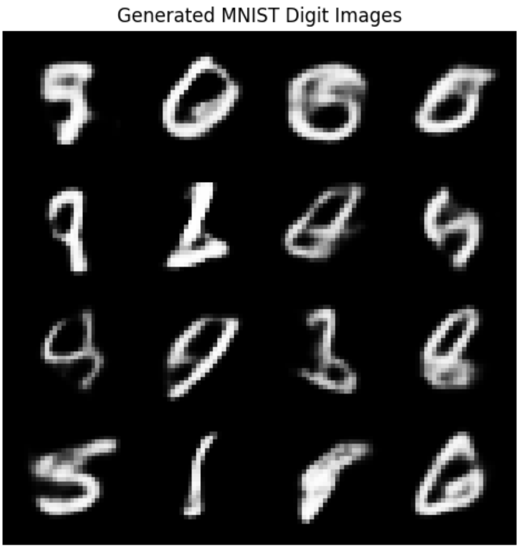
MNIST Digit Samples	MNIST Fashion Samples

---

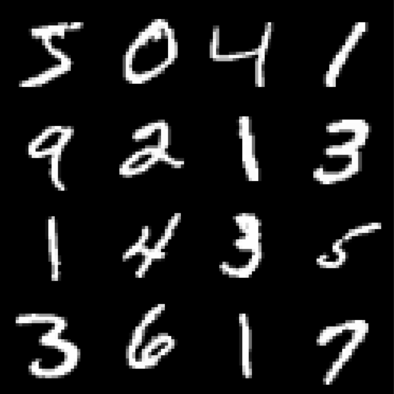Part 2: Implementing GANS

Following is the Neural architecture formed:

Info

Dropouts are particularly applied in Discriminator to underpower it and give Generator a chance to learn more thoroughly.

Declaring Hyperparameters

The following hyperparameters were declared:

• Latent Space Dimension = 100
• Image Shape = (1, 28, 28) | 1 Channel and 28 as both Width and Height
• Batch Size = 64
• Learning Rate = 0.0002
• Decay Rate = (0.5, 0.999)

Train the GAN on MNIST Digits

• Will use the Adam Optimizer with a the following decay rates:
  • ${\beta }_1$ as 0.5 and ${\beta }_2$ as 0.999
    • These parameters control how much weight is given to past gradients when computing the new weights using the parameter update equations
• Loss Function as Binary Cross Entropy (BCE) Loss
• Will shuffle the data when loading into the DataLoader
• In Training Phase:
  • The generator is made to produce images from random noises
  • The loss of the generator is calculated as the prediction of the discriminator for the generated image
    • If generated image predicted as real, low loss
    • If generated image predicted as unreal, high loss
  • The discriminator is made to predict both, real and fake images (generated by the generator) as real or fake
  • The loss of the discriminator is the mean of both result’s losses

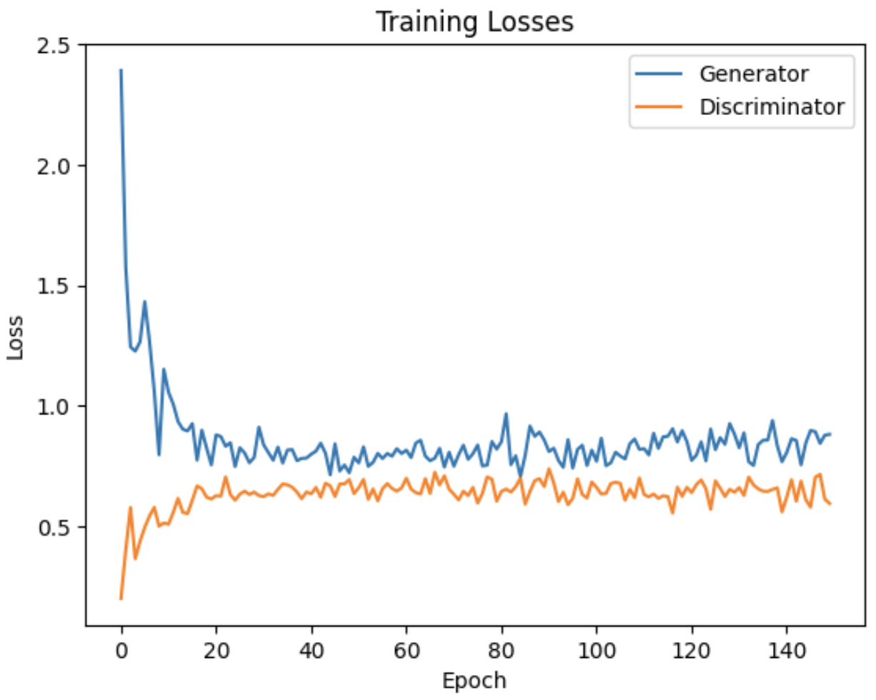
Following is the loss curve:

Train the GAN on MNIST Fashion

The training procedure will be the same as for Train the GAN on MNIST Digits.

Assumption

The GAN was trained on the entire MNIST Fashion dataset instead of just one class.
This was done so I could carefully analyze the Latent Space for different class labels and answer the questions in Part 4.
As for generating images for just one class label, I have deduced a method to do so. It will be elaborated in the report further.

Following is the loss curve:

Generate 10 Images from the Trained Generator

Following are the generated images from MNIST Digit Generator:

Following are the generated images from the MNIST Fashion Generator:

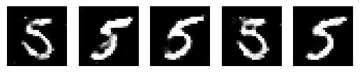
Generate 5 Images of Digit ‘5’ from the Trained Digit Generator

By analyzing the latent vectors corresponding to the digit “5”, we can generate new latent vectors close to these examples. We do this by adding small random noise or by linearly interpolating between the existing latent vectors. This helps explore the space around the original vectors to create variations of the same digit, allowing us to generate new images of “5” without manually specifying every detail. This method leverages the continuous nature of the latent space to create diverse yet similar outputs.

Following were the produced results:

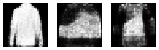
Generate Images of any one class from the Trained Fashion Generator

The chosen class is Shirt.

Using the same noise resampling technique as used in Generate 5 Images of Digit ‘5’ from the Trained Digit Generator, following are the results:

---

Part 3: Implementing VAE

Following the formed Neural architecture:

Declaring Hyperparameters

The following hyperparameters were declared:

• Latent Space Dimension = 22
• Image Shape = (1, 28, 28) | 1 Channel and 28 as both Width and Height
• Batch Size = 128
• Learning Rate = 0.001

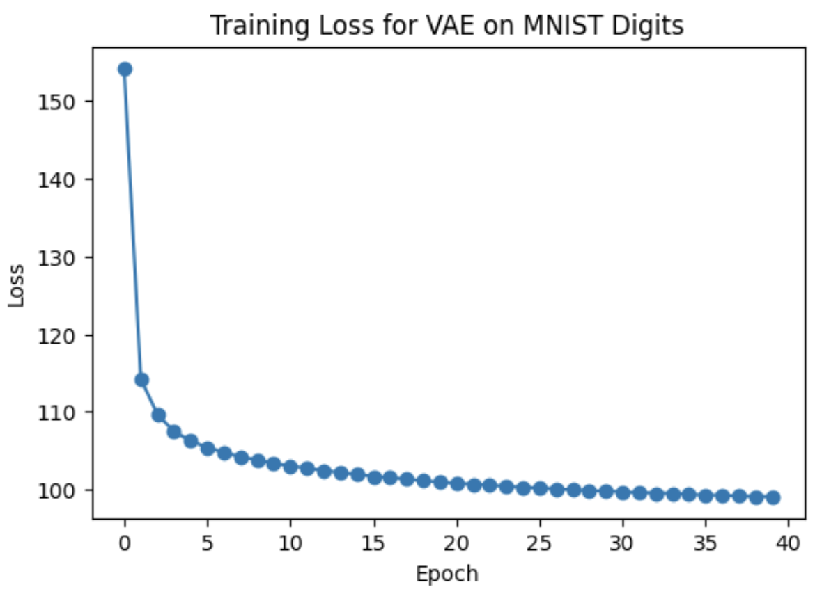
Train VAE on MNIST Digits

• Will use the Adam optimizer
• Data will be shuffle loaded
• During Training, for each data point:
  • Encoder processes the image and gives out its mean $\mu$ and log variance $\log {\sigma }^2$
  • The reparameterize function is then used to generate the latent vector z from the earlier mean and log variance: $z=\mu +ϵ\cdot \sigma$
  • Decoder after that uses the latent representation z to reconstruct the image
  • Reconstruction loss is then computed using Binary Cross Entropy Loss
  • KL Divergence loss is computed using its formula
  • Final loss is taken as the sum of both reconstruction and KL Divergence loss
  • Optimizer updates the parameters using the computed loss

Following is the loss curve:

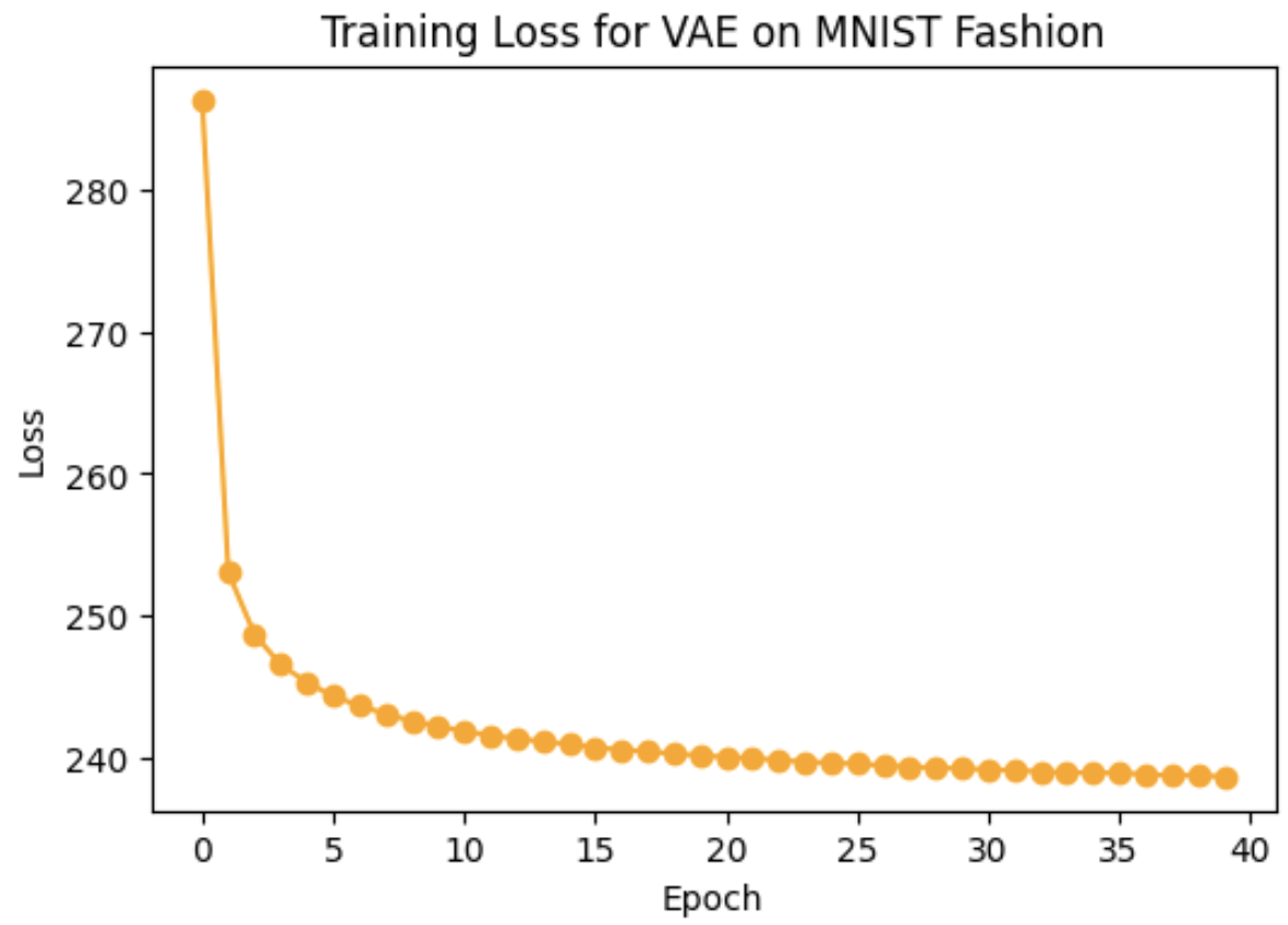
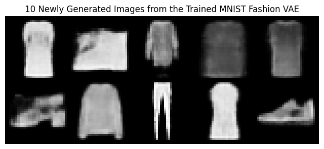
Train VAE on MNIST Fashion

The training procedure will be the same as for Train VAE on MNIST Digits.
The same assumption as in Train the GAN on MNIST Fashion was followed.

Following is the loss curve:

Visualize Latent Space using T-SNE

Sklearn’s Manifold package was utilized to visualize the latent space using T-SNE:

MNIST Digit Latent Space	MNIST Fashion Latent Space

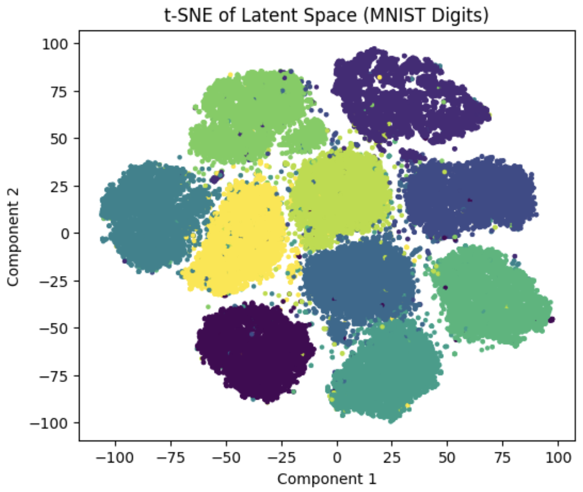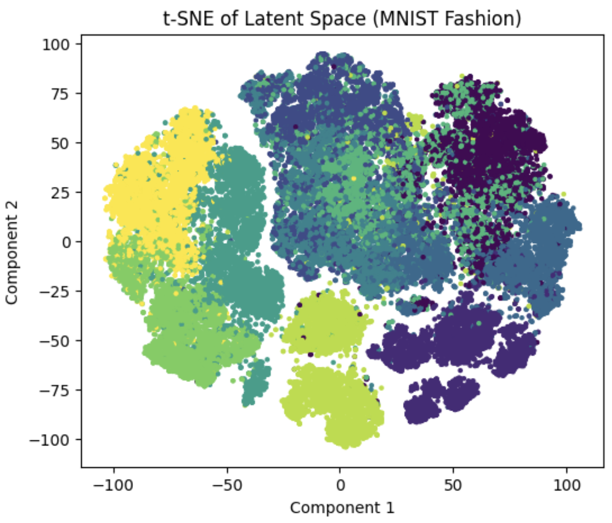Different color regions correspond to class labels represented by that latent region/space.
Therefore since we have about 10 class labels, the colors would also be 10 for both of the MNIST datasets.

Generate Digit Images through Sampled Latent Vectors

Latent vectors were sampled through a normal distribution and following were the results produced by the Decoder:

We can clearly see that the results can be improved. Through tampering, I found that increasing the epochs can significantly improve the generation quality.
The current trained epochs for the above result were 40. Training on more epochs can help us improve the generation quality.

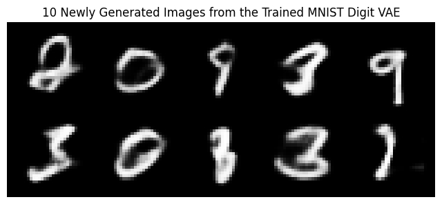
Generate 10 Images from the Trained VAE

Following images were generated via sampling the Latent Space:

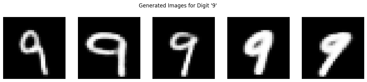
Generate 5 Images of the digit “9”

Tip

“9” is the last second digit of my roll no: 5695

While visualizing the latent space, the latent vectors for the images were stored against their labels. We can now take out latent vectors for specific class labels and then sample them to generate similar images. This strategy will be followed for both MNIST datasets.

Following are the generated images:

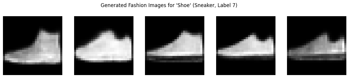
Generate Single Class Images from MNIST Fashion

We will choose the class “Shoe” this time.
The same technique as for Generate 5 Images of the digit “9” will be followed here.

Following are the resultant generated images:

---

Part 4: Comparison and Analysis

Here both, GAN and VAE will be compared in-terms of their weaknesses and strong points.

Image Quality: Which method generates clearer, more realistic digits?

Clearly, GAN generate more realistic and original looking images as compared to VAE.
This could be because VAE are supposed to compress the image data first, missing out on minute details and only reconstruct back to the image using major or prominent image features, resulting in a blurry and foggy image.

Training Stability: Which model was harder to train?

GAN was more difficult to train as compared to VAE. While VAE only required proper implementation of the architecture to get going, GAN on the other hand required intense hyperparameter analysis and right input / conditional values to properly minimize loss and generate promising results.

Latent Space: How do GANs and VAEs differ in learning latent spaces?

Due to its encoder-decoder architecture, VAE learn a more probabilistic and continuous latent space as compared to GAN which learns a non-probabilistic latent space. VAEs explicitly learn a structured latent space by enforcing a distributional constraint, leading to smooth interpolations and meaningful generative control. It is because of this distributional control that we can say VAEs produce blurrier images. GANs on the other hand implicitly learn a latent space without any explicit distributional constraints, resulting in more realistic images but with less interpretability and control over the latent space.

Potential Improvements with Respect to Hyperparameter Tuning

For both VAEs and GANs, a careful hyperparameter analysis is important.

Hyperparameter Improvements for VAE

The following things should be considered:

• Latent Dimension
  • A higher dimension captures complex variations but also make training harder and potentially lead to overfitting.
  • A smaller dimension forces the model to learn only the most salient features but might miss important details.
  • A balanced dimension is the key here so starting small and gradually increasing the dimension via reconstruction loss and other analysis can help.
• KL-Divergence / Reconstruction Loss
  • If the reconstructions are blurry then reducing the KL weight can help.
  • If the latent space is not well structured then increasing the KL weight can help.
• Learning Rate
  • Too high can under-fit the model and too low will slow convergence.
  • A sweat spot is from 0.001 and onwards in a small range.
• Batch Size
  • Larger batch sizes are preferred for more stable gradient estimates.

Hyperparameter Improvements for GAN

The following thing should be considered:

• Generator/Discriminator Balance
  • A powerful discriminator can overpower the generator (leading to vanishing gradients).
  • A weak discriminator may fail to provide meaningful feedback to the generator.
  • An optimal balance is a must between these two, just like in a MIN/MAX game.
  • Regularization of discriminator can help often .
• Learning Rate
  • GAN are highly sensitive to learning rates.
  • Both generator and discriminator should use the same learning rates and this should only change if discriminator keeps overpowering the generator
• Batch Size
  • Larger batch sizes can stabilize the training.
  • In our implementation, increasing the batch size can potentially improve our obtained results even more.
• Latent Dimension
  • Higher dimensional space can capture more complexity but might be harder to train.
  • The dimension used in our implementation as 100 and if increased can generate more promising results.

---

Part 5: Save the World with VAE

In this part, a real-life problem was to be identified and Variational Autoencoders were supposed to detect and help out in anomaly detection in such problems.

Problem / Potential Dataset

The problem highlighted in my case is the selling of defective medicines, particularly damaged tablets and capsules.
Many of the tablets and capsules generated in pharmaceutical industry are to filtered out and damaged ones are separated. This require careful analysis as even if one of the damaged capsule is sent to the market, not only will it incur monetary cost but also risk lives of the patients.

I plan to solve this problem with the help of VAE. A VAE which could carefully learn the structure of valid tablets and capsule can efficiently filter out the damaged or anomalous instances.

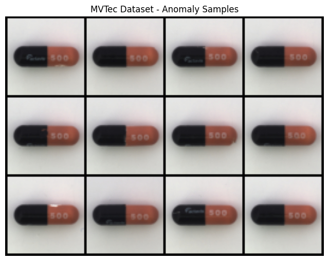
The data chosen in this case is the “Capsule” subset of the MVTecAD dataset. This dataset is used for benchmarking anomaly detection methods with a focus on industrial inspection. The subset of Capsule which I am working on contains about 219 training samples of various capsules in different shapes, labels and views.

Loading and Visualization of Data

The original capsule images were about 1000x1000 in resolution, however for optimal training and performance, I resized them to about 64x64 size.

Following are the visualizations of training/normal capsule samples:

Following are the visualizations of testing/defective capsule samples:

Architecture

As for the architecture of the VAE, a similar design was followed as made in Part 3 Implementing VAE. Though, there were some minor adjustments in the number and params of the Convolution layers to accommodate 3 channel (RGB) images. Lastly, the input image size and the decoder output image size was also adjusted accordingly to accommodate the current image characteristics.

The loss function was also the combination of KL Divergence and Binary Cross Entropy, as similar in Part 3 Implementing VAE.

Declaring Hyperparameters

Following hyperparameters were concluded to be the best for our data in hand:

• Batch Size = 8
• Learning Rate = 1e-3
• Latent Dim = 128
• Epochs = 20

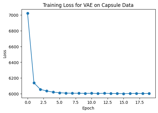
Training the Model on Capsule Images

The same training loop was followed as was in Part 3 Implementing VAE.

Following is the finalized loss curve:

Generation of Random Capsule Samples from VAE

Random capsule images were also generated from the trained VAE to understand the quality of the latent space and completeness of the features it was trained on.

Following were the generated results by the Decoder:

From here, we can conclude that the model was able to successfully learn the structure and distribution of Capsule images.

Testing Anomaly Correction

Now, we will provide our model with an anomalous sample and will make it reconstruct it using its learned latent space. This will get us an idea of what our model believes to be the right image.

Following are the results:

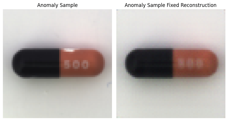
In this case, the anomalous capsule sample had the capsule broken in the image and our VAE model was able to reconstruct the image in such a way that the broken part was fixed. This highlights that the model is successfully able to detect the broken part of the capsule as an anomaly.

Anomaly Detection on Test Samples

Finally, we will conduct the anomaly detection on a single test sample to see the accuracy or detection power of our VAE model.

Testing Single Non-anomaly Sample

First, we will test one of the non-anomaly sample which the model has not already seen:
Following is the sample image:

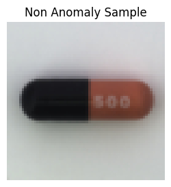
Following is the anomaly score and detection done by the VAE model on it:

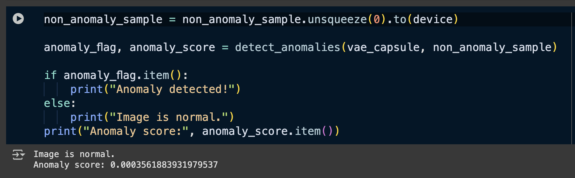
Good to Know

Since we are using Binary Cross Entropy Loss (BCE), the reconstruction loses and thus the anomaly scores are very low. This isn’t a problem and only required a low threshold to be chosen.

Testing Single Anomaly Sample

Next, we will feed the model an anomalous image which it has not seen before.
Following is the sample image:

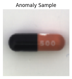
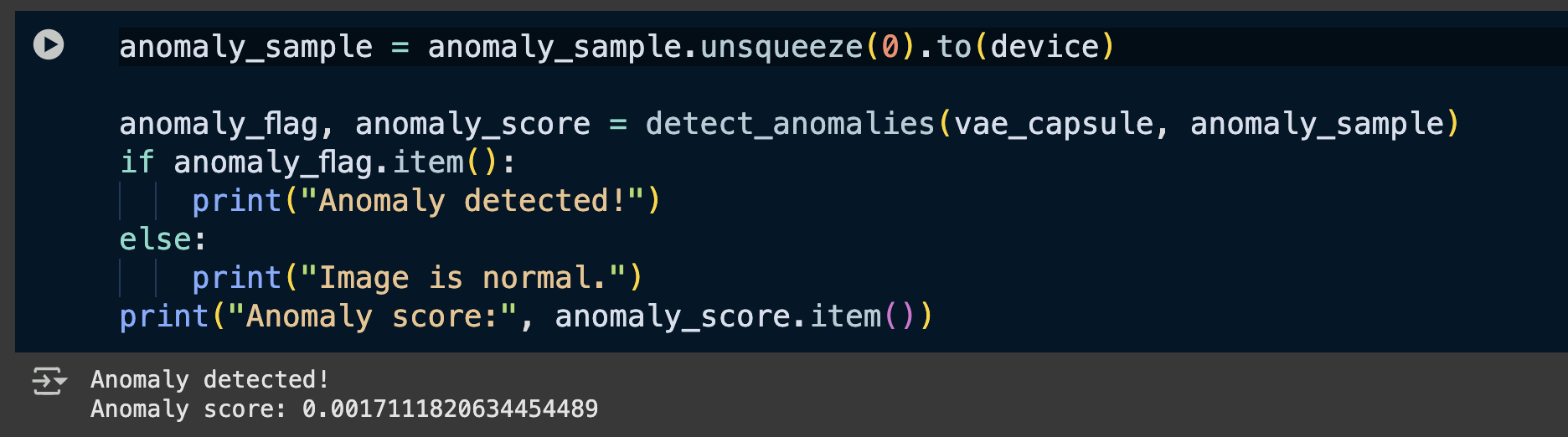
Following is the anomaly score and detection done by the VAE model on it:

Batch Anomaly Testing

Lastly, to conclude, we will test the anomaly detection on all of the anomalous test samples, which are not seen by the model.

Following are the final results:

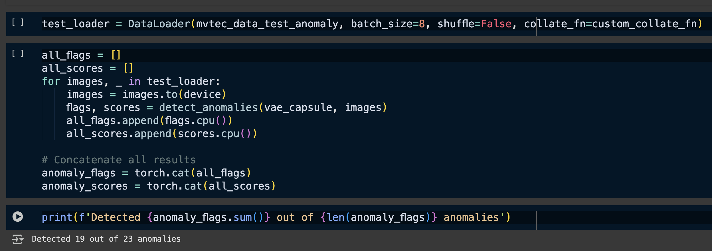
Results

We can clearly see that the model was about to correct detect as anomaly, 19 out of 23 anomalies. Therefore, on this small test dataset, the accuracy was around 82%.